International Journal of Electrical and Computer Systems (IJECS)

ISSN: 1929-2716

1. Introduction

On the 30th of November 2016, the European Commission published a key policy recommendations package, “Clean Energy for All Europeans”, sometimes referred to as the “Winter Package” [1]. The reforms contained various measures that encourage the implementation of some changes for power distribution and power transmission network management. These changes can be considered a transition from the so-called “power system management” to “power system self-management”.

For the most part, network control of conventional power systems is organized by partially automated dispatch control. The abundance of a huge variety of new renewable energy-based electricity generators complicates the dispatcher’s task in assessing the situation correctly, and making the right decision in time. Therefore, it is deemed appropriate to transfer some control tasks from the dispatcher to self-managed systems and controllers.

Electrical network load flow calculations are very time-consuming, this is primarily due to multiple iterations of calculation cycles, which are repeated until the required accuracy is achieved. The number of iterative cycles depends on the size and complexity of the electrical system [2]. The larger the electrical system, the greater the number of iterative cycles that are required. Therefore, a transformation of a large electrical network diagram to a smaller equivalent structure would speed up the analysis extensively.

Automatic computer decision-making can be successfully applied if the size of consumer loads and electricity-generating power sources are evaluated by their characteristics, and probability distributions of random variables of statistical significance. This in turn extends the decision-making time which further increases the demand for more efficient algorithms. In addition, the fast algorithms’ calculations can be used to identify the electromagnetic transients that are caused by short circuits to make the best possible fault elimination.

Fast automatic localization and isolation of damaged power line sections can protect power systems from possible blackouts [3]. This is very true in cases where power sources must be disconnected sequentially, depending on the character of the collapse.  This becomes very important for isolated and compensated power distribution networks when single phase earth faults occur [4].

2. Tasks of Stationary Mode Analysis for Real-Time Management

The duration of a load flow computer analysis increases in proportion to the complexity of the power system. This relates to the number of power lines and network diagram nodes [5].

Various difficulties of load flow calculations and comparison of load flow calculation methods have been discussed [6]. Due to the complexity of power systems being analyzed, which results in a long analysis time, the developed software is mainly used for educational and research activities, as well as for the planning of power systems [7 – 10]. The use of software, developed for real-time control of power system, is possible if the calculation and analysis times are sufficiently short to enable timely responses to change situations in the power system.

The analysis time can be shortened by an adequate simplification of the equivalent power network diagram. This includes the reduction of the number of nodes in the one-line diagram of power network.

Simplification of the complex network diagram in the developed and proposed technology is carried out in 3 main steps:

1. Sections of radial power network lines that have an intermediate load or generate connections sources, instead of converting every graph element of the line’s section, are converted into equivalent energy sources. This step is repeated until the radial branches are removed from the power network graph.
2. A list of basic power network graph nodes is then compiled.  The graph nodes in the basic power network are named after the ones that combine three or more remaining power network graph lines. If the power lines lie between two basic nodes and contain the intermediate energy sources, they are then replaced by an equivalent line. In such cases, the energy sources are transferred to the edges of the replaced line.
3. Finally, voltage values are found for each basic node of the simplified power network graph.

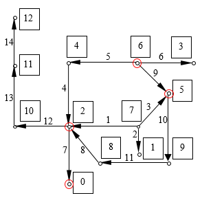
For the purpose of illustration, Figure 1(a) shows a part of the power line system that contains 15 lines and 13 nodes. Following Step 1, we can simplify the power system’s network graph by equivalently transferring the parameters of the largest branch number 15 to node number 10. Correspondingly, node number 13 disappears in the network graph, as shown in Figure 1(b).

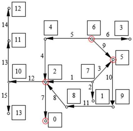
At the beginning of the first iteration, the voltage values of nodes 10 and 13 are set as the voltage of the balancing node (0).

The changes of the total rated power of the 10th node in the new network graph diagram then correspond to:

where:  is the initial value of the total power of node 10,  and  are the combined complex values of the total power in nodes 10 and 13, and  and  are the voltages of nodes 10 and 13.

The general formula for the first step simplification:

where:  is the power complex value of the node after simplification, P - active power,– imaginary unit.

After the first simplification, new radial lines can be formed. For example, as seen from the resulting network graph in Figure 1(b), a new line was formed from sections 12, 13, and 14. As a result, in the subsequent simplification of the network diagram, the parameters of these line sections replace the equivalent parameters of node 2.

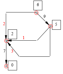
In Step 2, the line connections between the basic nodes are made equivalent by transferring the internal node parameters of the connections to the basic nodes. This results in a fully simplified network graph (Figure 3) where the basic nodes appear as 0, 2, 5, and 6. It is shown in Figure 2 that in addition to the equivalent transfer of node parameters (e.g. nodes 8 and 9 are transferred to nodes 2 and 5), the transfer of currents of the nodes and conductivities of energy sources can also be achieved.

After finding the voltages of the basic nodes from the nodes current in the simplified diagram, the voltages of all the nodes are then calculated in the load flow calculation task. All the steps of the task are repeated in iterative cycles until the required accuracy is reached. This means that the calculation time will be greatly lowered, having significantly reduced the number of computations and calls to RAM.

In order to evaluate the effectiveness of this simplification, the time required to reach the final solution of the task is compared with the conventional calculation methods. The matrix of nodal impedances has been found in advance allowing us to use nodal voltage detection in the computation time comparison:

where:  and matrixes of nodal voltages and currents,  - nodal impedances matrix.

For any node k, the nodal impedance is calculated as a conjunct value of ratio of full nodal power and nodal voltage:

The operations in these formulas are repeated at each iteration cycle. This means that the calculation time depends on the number of cycles and number of nodes in the network. Quite often in looped electrical networks, the number of lines is greater than the number of nodes. The examination of different power grids shows that the ratio between the number of lines to nodes is approximately 2. The higher this ratio is, the more iterations are required to achieve the desired accuracy in the application task. Table 1 classifies the network complexity level depending on the number of nodes and number of lines.

Table 1. Optimal number of nodes in the equivalent diagram.

1. Level of the network complexity	1	2	3	4	5
2. Number of nodes in the network	180	1180	2780	3930	5280
3. Number of lines in the network	320	2080	5440	7720	10400
4. Number of nodes after simplification	12	32	52	62	72

A conditional match between the level of complexity (row 1), the nodes of a network diagram, and the number of lines (rows 2 and 3) was accepted. The optimal simplification degree was found for the appropriate complexity level of the power system with respect to the computation time. Such standard calculations for the cyclic procedure required us to find voltages in the remaining nodes of the equivalent scheme, requiring significant periods of time. The «spreading» of found voltages and their transfer to all nodes of the basic network were also taken into consideration. Corresponding optimal numbers of equivalent diagram nodes are presented in Table 1 (row 4).

The duration of network load flow calculations using the conventional method and the simplified equivalent system, are shown in Figure 3. In this graph, the upper curve illustrates the effect of using the conventional calculation, whereas the lower curve shows the computation time after simplification. The curve clearly indicates that the computational time increases with rising network complexity.

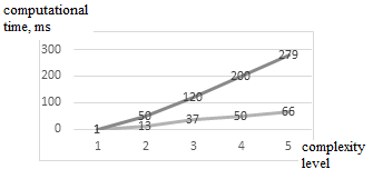
Figure 4 shows the computation time dependence on the level of complexity of network diagram, in cases when the equivalent schema was used. The calculations were done on a computer with a 2.8 GHz CPU.

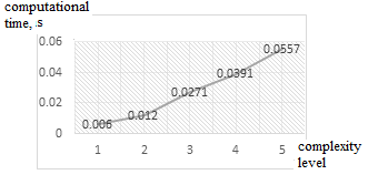
Although the difference in calculation time for different complexity levels varies by about a factor of 10, and the longest calculation time is less than 1 second, it should be noted, that the results of computation given in the figures (3 and 4) are for single deterministic computation. In probabilistic computations, when evaluating many different power system performance statuses, particular in emergency cases, in order to find the most appropriate solution, it will be necessary to perform a lot of deterministic computations. Therefore, for real-time management, it is important to have the shortest computational time as possible.

The data suggests that more efficient algorithms for electrical network management computations can significantly reduce the computation time. Other benefits of using diagram simplification technology include acceleration of short circuit calculations and reduction of RAM usage. Typically, such calculations are performed after load flow analysis, having already identified the voltages of the stationary mode for the network diagram nodes. In the succeeding step, the task is supplemented by an addition of the internal impedances of the generating sources and loads in each node of the network diagram. The impedances acquired from the voltages in the preliminary load flow calculations allow us to determine the k^th node’s currents, :

where:    - admittance of the load or energy generating source; - internal impedance.

For example, we can then equate the internal conductivities of the 15^th branch (refer to the Figure 1, Step 1) by the residual conductivity of node 10, which can be found as follows:

where:  is previous value of the conductivity.

The equivalent current of node 10 can be subsequently found:

where: is previous value of the current.

The accelerated load flow and short circuit calculation algorithms form the basis of a software program that can be used for power system dynamic stability research.

The calculated values of powers  and voltages  of nodes with synchronous generators in the load flow calculation task enables us to calculate the stationary mode initial voltage of the emf and the power required from the generator's turbine. This corresponds to:

where:  and  are the initial electromotive voltage and electric power of generator respectively, before the start of the electromechanical transients process and after the switching excess in power network.

After the mechanical rotation of the generators in relation to the magnetic fields of the stator, due to the altered electric power: , the algorithm allows us to find the short circuit calculations, at a discrete time step, the new values of the node currents, :

The calculation algorithm is accelerated by using the equivalent diagram in calculations. This reduces the duration of the analysis of the electromechanical processes. For example, on the occasion when the system reaches the 5^th level of complexity and the discrete step in the mechanical generator is set to 0.1 seconds, the simulation of the real 1-minute action takes up less than 50 seconds. This value is comparatively smaller than the duration of the real action itself, and even more so for the 1-hour simulation, for which formulas (3-7) were used.

2.1. Control of Reactive Load Flow by Reactors

The reactive load flow control of the power system can be exceptionally useful at the initial phase of the network management performance, as estimated by the quantities of the connecter shunt reactor and capacitor banks, or by synchronous compensators [11, 12]. For such equipment, a fast management system is not necessary. By contrast, the choice of equipment is complicated by switching of occasional users and the generated power change. Up to 1,000 statistical test calculations must be performed if the energy consumption is accidental in nature and distributed generation is integrated into the power system. This occurs either by the selection of compensating means, limiting voltages up to the acceptable values or minimizing power losses. But even in such cases, the equivalent simplification of power network reduces the calculation time down to a few seconds. As a result, such computer technology can successfully serve to advise the dispatcher during the initial stages of network management.

3. Models of Electromagnetic Transients for Real-Time Management

In addition to the stationary mode control, a rapid search for the optimal and dynamically stable system structures must be carried out by the automatic dispatcher. It facilitates the important analysis task and ensures that the short circuit modes will be less time-consuming. The founded power load flow distribution dictates the necessity of iterative cycles. Here, a single line diagram can also be successfully simplified in the load flow calculation task. On the other hand, it is observed that during the electromechanical process calculation, whenever the process monitoring of the discrete times steps is used, computation time increases for each iteration. The performed analysis has shown a possibility that the calculation time would not exceed a few tens of milliseconds.

In such tasks, fast electromagnetic processes are being solved when it is necessary to determine the character of short circuits, the cause of the fault and the distance to the fault in the line. After emergency failures, it is essential to determine the reliability indices of possible network structures, based on the insulation damages evaluated by overvoltage. The voltage processes and their amplitudes after switching depend on many factors. These include initial phases at the switching moment, residual charges, and the impedance at the fault spot among others. The evaluation of these factors by random variables in necessary, this repetition significantly prolongs calculations. Therefore, the events analysis algorithm is much faster.

Acceleration of calculations in the software of electromagnetic transient processes is achieved by separating the mathematical modelling procedures from the preparation of the initial parameters. In such procedures, various types of digital filters and matrix differential equations are used.

Previous studies have shown [13, 14], that the shortest computation time is achieved when modelling overhead lines and cables with wave equations. Suitable wave attenuation and the change of surge impedance are achieved by digital filters that are optimized with the frequency spectrum.

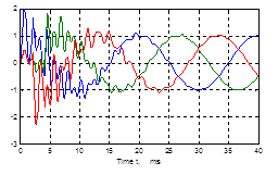
Figure 5 illustrates the voltage curve after applying a switching operation to a 50 km long power line. The voltage change curve shows that when the switching operation is performed with phase connection at different times, the asymmetry may arise from the merger moments of different circuit breakers. Hence, modelling time with no more than 0.04 seconds for one power frequency period is achieved.

The choice of an example with overvoltage line switching deliberately draws the attention to the implementations in the program i.e. to the peculiarities of the formation of the initial part of the overvoltage switching. In most cases, when transient processes in power lines are simulated by wave equations, surge impedances of power line’s wave channels are considered to be constant over time [15].  Practical modelling shows that surge impedance is variable in initial moment of transient [16]. The assumption, that surge impedance is considered to be constant over time, although the surge impedance actually changes rapidly, calculates up to 10% error in the ratio between currents and voltages in the wave channels at the transient initial moment. In the transient calculation algorithm, this surge impedance change is described by introducing the frequency function of such a change and its transformation into a transient characteristic in a time dimension.

The line wave equation for one wave channel, written with relation to the beginning of the line, is composed in the algorithm as follows:

where: and  – voltage at the beginning and end of the line;  – current at the beginning of the line;  and  - an voltage wave reaching the beginning of the line and the end of the line;  –  surge impedance of ideal (without losses ) power line; l and v – length of power line and velocity of surface electromagnetic wave propagation;  and  - electromagnetic wave propagating in the line damping factor and     surge impedance change factor;

represents the convolution of two-time functions.

For example, a convolution of  and  time functions can be performed by a digitalized integral:

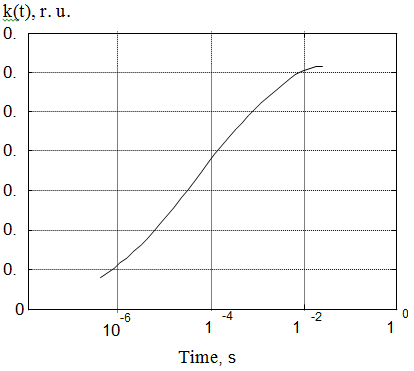
Figure 6 shows a function of the change in time factor of surge impedance in the channel, also known as “wires - the earth”. The specific resistivity of the ground soil under 110 kV power line equals to 100 ohms. From the displayed graph, we observe that the essential change of surge impedance occurs the during the first microseconds, therefore, changing the initial view of the electromagnetic processes substantially.

4. Conclusions

• A developed methodology for simplification and return to the previous structure of complex power networks (up to 10,000 lines and 5,000 substations), when the network elements are replaced by corresponding equivalents, have been shown to significantly speed up the following processes: the computer analysis of stationary process in the load flow calculations, short circuit calculations and electromagnetic transients analysis.
• Simplified electricity network load flow calculations can be carried out using known load flow calculation methods.
• By using the equivalents of power network compensating tools for effective load flow management, computation time, as well as the probabilistic assessments of network load and generated power can all be reduced up to several seconds. This computation period is sufficient because the compensating tools used are not fast acting devices.
• For insulation coordination, identifying network failures and for rapid fault localization, it is appropriate to use the electromagnetic transient modelling by applying power line wave equations with a widespread use of a variety of digital filters.

References

[1] Eurelectric’s Key Policy Recommendations Winter Package Solutions, Union of the Electricity Industry, Belgium, Brussels, 2016. [Online]. Available: http://www.eurelectric.org/media/293202/winter_package_solutions-2016-030-0496-01-e.pdf. View Article.
[2] R. Franke and H. Wiesmann, “Flexible modeling of electrical power systems - the Modelica PowerSystems library,” Modelica Conference, Lund, Sweden, 2014. View Article
[3] G. Beck, et al, Global Blackouts – Lessons Learned, 2005, POWER-GEN Europe 2005, Milan, Italy June 28 – 30, 2005, [Online]. Available: http://www.energy.siemens.com/us/pool/hq/power-transmission/HVDC/Global_Blackouts.pdf. View Article
[4] L. Rui, et al, “Research of Fault Location in Distribution Networks Based on Integration of Travelling Wave Time and Frequency Analysis [J],” Proceedings of the CSEE, 28, pp. 130-136, 2013.
[5] J. J. Deng, H. D. Chiang, “Convergence Region of Newton Iterative Power Flow Method: Numerical Studies,” Journal of Applied Mathematics, vol. 2013, 2013. View Article
[6] O. A. Afolabi, et al, “Analysis of the Load Flow Problem in Power System Planning Studies,” Energy and Power Engineering, pp. 509-523, 2015. [Online]. Available: http://www.scirp.org/journal/epe. View Article
[7] MATLAB. [Online]. Available: https://www.mathworks.com/products/matlab.html (Computer software). Visit Website
[8] RADIRING Software – Student Version 1.1, 2015. (Computer software).
[9] ETAP, [Online]. Available: https://etap.com/product/load-flow-software (Computer software). Visit Website
[10] PSS®SINCAL, [Online]. Available: http://w3.siemens.com/smartgrid/global/en/products-systems-solutions/software-solutions/planning-data-management-software/planning-simulation/pss-sincal/pages/pss-sincal.aspx (Computer software). Visit Website
[11] K. Papp, et al “High Voltage Series Reactors for Load Flow Control,” CIGRE, pp. C2-206, 2004. [Online]. Available: http://www.cigre.org. View Article
[12] C. Bengtsson, et al, “Dynamic Compensation of Reactive Power by Variable Shunt Reactors - Control Strategies and Algorithms,” CIGRE, pp. C1-303, 2012.
[13] A. Semlyen, A. Dabuleanu, “Fast and accurate switching transient calculations on transmission lines with ground return using recursive convolutions,” IEEE Transactions on Power Apparatus and Systems, vol. 94, no. 2, pp. 561-571, 1975. View Article
[14] A. Semlyen, “Ground return parameters of transmission lines an asymptotic analysis for very high frequencies,” IEEE Transactions on Power Apparatus and Systems, vol. PAS-100, pp. 1031-1038, 1981. View Article
[15] J. A. Martinez-Velasco, B. Gustavsen, “Overview of overhead line models and their representation in digital simulations,” 4th IPST, Rio de Janeiro, Brazil, 2001.
[16] M. V. Kostenko, L. S. Perelman, “K rasčetu volnovych processov v mnogoprovodnych linijach,” Izvestija, AN SSSR. Energetika i transport, no. 6, 1963.