International Journal of Electrical and Computer Systems (IJECS)
ISSN: 1929-2716

Volume 1, Issue 1, Year 2012 - Pages 1-8
DOI: 10.11159/ijecs.2012.001
Constrained Nonlinear Least Squares: A Superlinearly Convergent Projected Structured Secant Method
Nezam Mahdavi-Amiri, Narges Bidabadi
Sharif University of Technology, Faculty of Mathematical Sciences
Azadi Street, Tehran, Iran
nezamm@sina.sharif.edu, n_bidabadi@mehr.sharif.ir
Abstract - Numerical solution of nonlinear least-squares problems is an important computational task in science and engineering. Effective algorithms have been developed for solving nonlinear least squares problems. The structured secant method is a class of efficient methods developed in recent years for optimization problems in which the Hessian of the objective function has some special structure. A primary and typical application of the structured secant method is to solve the nonlinear least squares problems. We present an exact penalty method for solving constrained nonlinear least-squares problems, when the structured projected Hessian is approximated by a projected version of the structured BFGS formula and give its local two-step Q-superlinear convergence. For robustness, we employ a special nonsmooth line search strategy, taking account of the least squares objective. We discuss the comparative results of the testing of our programs and three nonlinear programming codes from KNITRO on some randomly generated test problems due to Bartels and Mahdavi-Amiri. Numerical results also confirm the practical relevance of our special considerations for the inherent structure of the least squares.
Keywords: Constrained Nonlinear Least Squares, Exact Penalty Methods, Projected Hessian Updating, Structured Secant Updates, Two-Step Superlinear Convergence
© Copyright 2012 Authors - This is an Open Access article published under the Creative Commons Attribution License terms. Unrestricted use, distribution, and reproduction in any medium are permitted, provided the original work is properly cited.
1. Introduction
Consider the constrained nonlinear least squares (CNLLS) problem,
where, ![]() ,
, ![]() ,
, ![]() ,
, ![]() , and
, and![]() ,
, ![]() , are
functions from
, are
functions from ![]() to
to![]() , all assumed
to be twice continuously differentiable. These problems arise as experimental
data analysis problems in various areas of science and engineering such as
electrical engineering, medical and biological imaging, chemistry, robotics,
vision, and environmental sciences; e.g., see Nievergelt (2000), Golub and
Pereyra
(2003) and Mullen et al. (2007). The gradient and Hessian of
, all assumed
to be twice continuously differentiable. These problems arise as experimental
data analysis problems in various areas of science and engineering such as
electrical engineering, medical and biological imaging, chemistry, robotics,
vision, and environmental sciences; e.g., see Nievergelt (2000), Golub and
Pereyra
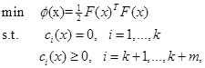
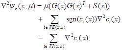
(2003) and Mullen et al. (2007). The gradient and Hessian of ![]() can be expressed as
can be expressed as
and
where, ![]() is the matrix whose columns are the
gradients
is the matrix whose columns are the
gradients![]() , and
, and
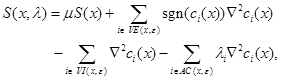
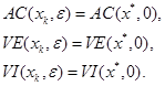
Using this special structure for approximating the Hessian matrix has been the subject of numerous research papers; see Fletcher and Xu (1987), Dennis et al. (1989), Mahdavi-Amiri and Bartels (1989), Li et al. (2002), Mahdavi-Amiri and Ansari (2012a), and Bidabadi and Mahdavi-Amiri (2012). Here, we consider the structured BFGS approximate formula (Dennis et al., 1989) for the structured least squares projected Hessian and a special line search scheme given by Mahdavi-Amiri and Ansari (2012c) leading to a more efficient algorithm than general nonlinear programming schemes. An exact penalty function for nonlinear programming problems is defined to be
where, ![]() is a penalty parameter. If
is a penalty parameter. If ![]() is a stationary point of (1) and the
gradients of the active constraints at
is a stationary point of (1) and the
gradients of the active constraints at ![]() are
linearly independent, then there exists a real number
are
linearly independent, then there exists a real number ![]() such
that
such
that ![]() is also a stationary point of
is also a stationary point of![]() , for each
, for each![]() . Mahdavi-Amiri and Bartels (1989), based
on a general approach for nonlinear problems (See Coleman and Conn, 1982a),
proposed a special structured algorithm for minimization of
. Mahdavi-Amiri and Bartels (1989), based
on a general approach for nonlinear problems (See Coleman and Conn, 1982a),
proposed a special structured algorithm for minimization of ![]() with a fixed value of
with a fixed value of ![]() in solving the CNLLS
problems. Let
in solving the CNLLS
problems. Let ![]() be a small
positive number used to identify the near-active (
be a small
positive number used to identify the near-active (![]() -active)
constraint set. The algorithm obtains search directions by using an
-active)
constraint set. The algorithm obtains search directions by using an ![]() -active set
-active set

and a corresponding merit function:
where,
Step lengths are chosen
by using![]() , which is
, which is ![]() with
with![]() . The optimality conditions are checked by
using
. The optimality conditions are checked by
using![]() , as well. The gradient and Hessian of
, as well. The gradient and Hessian of ![]() are:
are:
and
where,
It is well known that
the necessary conditions for ![]() to be an isolated local
minimizer for
to be an isolated local
minimizer for![]() , under the assumptions made above on
, under the assumptions made above on ![]() and the
and the![]() , are
that there exist multipliers,
, are
that there exist multipliers, ![]() , for
, for![]() , such that
, such that
A point ![]() for which only (12) above is satisfied is
called a stationary point of
for which only (12) above is satisfied is
called a stationary point of![]() . A minimizer
. A minimizer ![]() must be a stationary
point satisfying (13). One major premise of the algorithm is that the
multipliers are only worth estimating in the neighborhoods of stationary
points. Nearness to a stationary point is governed by a stationary tolerance
must be a stationary
point satisfying (13). One major premise of the algorithm is that the
multipliers are only worth estimating in the neighborhoods of stationary
points. Nearness to a stationary point is governed by a stationary tolerance![]() . The algorithm is considered to be in a
local state, if norm of the projected or reduced gradient, i.e.,
. The algorithm is considered to be in a
local state, if norm of the projected or reduced gradient, i.e.,![]() , is smaller than this tolerance, and it is
in a global state, otherwise. Fundamental to the approach is the following
quadratic problem:
, is smaller than this tolerance, and it is
in a global state, otherwise. Fundamental to the approach is the following
quadratic problem:
where,
the ![]() are the Lagrange multipliers associated
with (14) in a local state (in the proximity of a stationary point) and the
are the Lagrange multipliers associated
with (14) in a local state (in the proximity of a stationary point) and the ![]() are taken to be zero when the algorithm is
in a global state (far from a stationary point). In practice, the QR
decomposition of
are taken to be zero when the algorithm is
in a global state (far from a stationary point). In practice, the QR
decomposition of ![]() is used to solve the quadratic
problem:
is used to solve the quadratic
problem:
If we set ![]() , for some
, for some ![]() , then
, then ![]() is to be found by solving
is to be found by solving
Therefore, for solving
the quadratic problem (14), we need an approximation for the projected or
reduced Hessian ![]() . We are to present a
projected structured BFGS update formula for computing an approximation
. We are to present a
projected structured BFGS update formula for computing an approximation ![]() by providing
a quasi-Newton approximation
by providing
a quasi-Newton approximation![]() , where,
, where,
with the setting ![]() . We give the asymptotic convergence
results of exact penalty methods using this projected structured BFGS updating
scheme. Consider the asymptotic case, that is, the case that the final active
set has been identified, so that for all further
. We give the asymptotic convergence
results of exact penalty methods using this projected structured BFGS updating
scheme. Consider the asymptotic case, that is, the case that the final active
set has been identified, so that for all further ![]() , with
, with ![]() designating the optimal point, we have
designating the optimal point, we have
Suppose that
and we want to update ![]() to
to ![]() ,
approximating
,
approximating
Note that![]() , where
, where ![]() is the
number of active constraints. We assume rank (
is the
number of active constraints. We assume rank (![]() ) =
) =![]() , for all
, for all![]() . Letting
. Letting ![]() and
and ![]() , we have
, we have ![]() , where, in order to simplify notation,
the presence of a bar above a quantity indicates that it is taken at iteration
, where, in order to simplify notation,
the presence of a bar above a quantity indicates that it is taken at iteration ![]() , and the absence of a bar indicates
iteration
, and the absence of a bar indicates
iteration ![]() . If the constraints are linear, then
. If the constraints are linear, then![]() , for
, for![]() . In the
nonlinear case, asymptotically it is expected that
. In the
nonlinear case, asymptotically it is expected that ![]() be
negligible and thus we obtain (Mahdavi-Amiri and Bartels, 1989):
be
negligible and thus we obtain (Mahdavi-Amiri and Bartels, 1989):
Thus, we use the
quasi-Newton formula to update ![]() to
to ![]() according to the secant equation
according to the secant equation![]() , when
, when ![]() has actually
become negligible, that is, when
has actually
become negligible, that is, when
for![]() , where
, where ![]() is the
iteration number and
is the
iteration number and ![]() denotes the
Euclidean norm, as suggested by Nocedal and Overton (1985) for general
constrained nonlinear programs. Therefore, an approximation
denotes the
Euclidean norm, as suggested by Nocedal and Overton (1985) for general
constrained nonlinear programs. Therefore, an approximation ![]() to
to ![]() is
is
where,
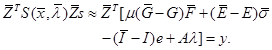
A general framework for exact penalty algorithm to minimize (5) is given below (see Mahdavi-Amiri and Bartels, 1989).
Algorithm 1: An Exact Penalty Method.
Step 0: Give an
initial point ![]() and
and ![]() .
.
Step 1: Determine![]() ,
, ![]() ,
,![]() ,
, ![]() . Identify
the matrix
. Identify
the matrix ![]() by computing the QR decomposition of
by computing the QR decomposition of ![]() and set global=true, optimal=false.
and set global=true, optimal=false.
Step 2: If ![]() , then obtain the search direction
, then obtain the search direction ![]() that is a solution of the quadratic
problem (14), where,
that is a solution of the quadratic
problem (14), where, ![]() approximates the global
Hessian
approximates the global
Hessian ![]() , and go to Step 5.
, and go to Step 5.
Step 3: Determine the
Lagrange multipliers![]() ,
, ![]() , as a solution of
, as a solution of
If conditions (13) are
not satisfied, then choose an index ![]() for which
one of (13) is violated, and determine the search direction
for which
one of (13) is violated, and determine the search direction ![]() that satisfies the system of equations
that satisfies the system of equations ![]() , where,
, where, ![]() is the
is the ![]() th unit vector, and
th unit vector, and ![]() , and go to Step 5.
, and go to Step 5.
Step 4: Set
global=false. Determine the direction ![]() , where,
, where, ![]() is the solution to the quadratic problem
(14),
is the solution to the quadratic problem
(14), ![]() approximates the local Hessian
approximates the local Hessian ![]() with
the
with
the ![]() being the Lagrange multipliers
associated with (14) as determined in Step 3. The vertical direction
being the Lagrange multipliers
associated with (14) as determined in Step 3. The vertical direction ![]() , is the solution to the system
, is the solution to the system
where, ![]() is the vector of the constraint
functions, ordered in accordance with the columns of
is the vector of the constraint
functions, ordered in accordance with the columns of ![]() .
Set
the step length
.
Set
the step length ![]() and go to Step 6.
and go to Step 6.
Step 5: Determine
step length ![]() using a line search procedure on
using a line search procedure on ![]() .
.
Step 6: Compute ![]() . If a sufficient decrease has been
obtained, then set
. If a sufficient decrease has been
obtained, then set ![]() , else go to Step 8.
, else go to Step 8.
Step 7: If
global=false, then check the optimality conditions for ![]() . If
. If ![]() is optimal, then set optimal=true and
stop, else go to Step 1.
is optimal, then set optimal=true and
stop, else go to Step 1.
Step 8: If
global=true and ![]() , then reduce
, then reduce ![]() to change
to change ![]() , else reduce
, else reduce
![]() so that
so that ![]() becomes
large tested against
becomes
large tested against ![]() .
.
Step 9: If
(global=true and ![]() ) or
) or ![]() is too small or
is too small or ![]() is too
small, then report failure and stop, else go to Step 1.
is too
small, then report failure and stop, else go to Step 1.
Remarks: In Step 6, we
have used an appropriate nonsmooth line search strategy to determine the step
length satisfying a sufficient decrease in ![]() that is
characterized by the line search assumption; see Coleman and Conn (1982b), part
(v), P. 152. For a recent line search strategy for CNLLS problems, see
Mahdavi-Amiri and Ansari (2012a, 2012c). In Step 7, the optimality conditions
are checked as follows: If
that is
characterized by the line search assumption; see Coleman and Conn (1982b), part
(v), P. 152. For a recent line search strategy for CNLLS problems, see
Mahdavi-Amiri and Ansari (2012a, 2012c). In Step 7, the optimality conditions
are checked as follows: If ![]() is small
enough, then determine the multipliers
is small
enough, then determine the multipliers ![]() ,
, ![]() , as the least squares solution of (26).
If the conditions (13) are satisfied, then
, as the least squares solution of (26).
If the conditions (13) are satisfied, then ![]() is considered
to satisfy the first order conditions, and thus
is considered
to satisfy the first order conditions, and thus ![]() being a
stationary point, the algorithm stops, as commonly practiced in optimization
algorithms. Of course, second order conditions are needed to be checked to
ascertain optimality of
being a
stationary point, the algorithm stops, as commonly practiced in optimization
algorithms. Of course, second order conditions are needed to be checked to
ascertain optimality of ![]() .
.
In the remainder of our
work, we drop the index ![]() from
from ![]() and
and ![]() , for
simplicity.
, for
simplicity.
For approximating the
projected structured Hessians in solving the quadratic problem, we make use of the
ideas of Dennis et al. (1989) in a different context. We consider the
structured BFGS update of ![]() , given by
, given by
where,
 and
and
Remark: Clearly, ![]() , given by (32), satisfies the secant
equation
, given by (32), satisfies the secant
equation ![]() .
.
Here, we use the BFGS secant updates for approximating the projected structured Hessians in solving the constrained nonlinear least squares problem.
The remainder of our work is organized as follows. In § 2, we give the asymptotic two-step superlinear convergence of the algorithm. Competitive numerical results are reported in § 3. The results are compared with the ones obtained by the three algorithms in the KNITRO software package for solving general nonlinear programs. We conclude in § 4.
2. Local Convergence
Here, we give our local two-step superlinear convergence result. We make the following assumptions.
Assumptions:
(A1) Problem (1)
has a local solution![]() . Let
. Let![]() .
.
(A2) ![]() , generated by Algorithm 1 for minimizing
, generated by Algorithm 1 for minimizing
![]() is so that
is so that ![]() ,
, ![]() .
.
(A3) The function
![]() and
and ![]() ,
, ![]() , are twice continuously differentiable
on the compact set
, are twice continuously differentiable
on the compact set ![]() .
.
(A4) ![]() and
and ![]() are locally Lipschitz
continuous at
are locally Lipschitz
continuous at ![]() .
.
(A5) ![]() is locally Lipschitz continuous at
is locally Lipschitz continuous at ![]() , that is, there exist a constant
, that is, there exist a constant ![]() such that
such that
(A6) The
gradients of the active constraints at ![]() , for all
, for all ![]() , are linearly independent on
, are linearly independent on ![]() .
.
(A7) There exist
positive constants ![]() and
and ![]() such that
such that
where, ![]() is the projected Hessian at
is the projected Hessian at ![]() .
.
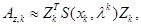
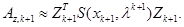
We will make use of the following two theorems from Mahdavi-Amiri and Ansari (2012a) and Nocedal and Overton (1985).
Theorem 1.
(Mahdavi-Amiri and Ansari, 2012a) There exists ![]() such that if
such that if ![]() and
and ![]() , then
, then
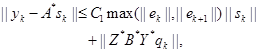
where, ![]() ,
, ![]() is a
constant independent of
is a
constant independent of ![]() , and if equation (8)
holds, then
, and if equation (8)
holds, then
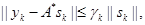
where,
and ![]() .
.
Theorem 2. (Nocedal and
Overton, 1985) Suppose that Algorithm 1 is applied with any update rule for
approximating the projected Hessian matrix. If ![]() ,
,![]() , for all
, for all ![]() , and
, and
then ![]() , at a two-step Q-superlinear rate.
, at a two-step Q-superlinear rate.
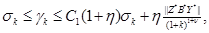
We now give the so-called bounded deterioration inequality for the structured BFGS update formula.
Theorem 3. Suppose that
the inequality (23) and Assumptions (A5) and (A7) hold. Let ![]() be the projected structured BFGS secant
update formula, that is,
be the projected structured BFGS secant
update formula, that is, ![]() where,
where, ![]() is the BFGS update formula of
is the BFGS update formula of ![]() obtained by using (28). Then, there
exist a positive constant
obtained by using (28). Then, there
exist a positive constant ![]() and the neighborhood
and the neighborhood ![]() such that
such that
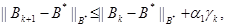
for all![]() .
.
Now, we give a linear convergence result.
Theorem 4. Suppose that
Assumptions (A1)-(A7) hold. Let ![]() be the structured BFGS
secant update formula, that is,
be the structured BFGS
secant update formula, that is, ![]() where,
where, ![]() is the BFGS update formula of
is the BFGS update formula of ![]() obtained by using (28). Let the sequence
obtained by using (28). Let the sequence
![]() be generated by Algorithm 1. For any
be generated by Algorithm 1. For any ![]() , there exist positive constants
, there exist positive constants ![]() and
and ![]() such that if
such that if
![]() and
and ![]() , then
, then
that is, ![]() converge to
converge to ![]() , at least at
a two-step Q-linear rate.
, at least at
a two-step Q-linear rate.
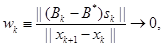
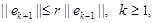
The next theorem shows the satisfaction of (34) in Theorem 2 for the structured BFGS update formula.
Theorem 5. If ![]() exists so that for every iteration
exists so that for every iteration ![]() , we have
, we have

and we update the ![]() using the structured BFGS secant formula
for each
using the structured BFGS secant formula
for each ![]() , that is,
, that is, ![]() ,
where,
,
where,
![]() is the BFGS update formula of
is the BFGS update formula of ![]() obtained by using (28), then
obtained by using (28), then
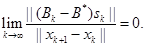
In §1, we pointed out that we use the structured quasi-Newton update formula for approximating the projected Hessian in Algorithm 1, if the inequality (23) holds (this is expected to happen when the algorithm is in its local phase with the iterate being close to a stationary point). Now, we give the superlinear convergence result for Algorithm 1.
Theorem 6. Suppose that
Assumptions (A1)-(A7) hold. Let the sequence ![]() be generated
by Algorithm 1 and
be generated
by Algorithm 1 and ![]() be obtained by
be obtained by
where, ![]() is the BFGS update formula of
is the BFGS update formula of ![]() obtained by using (28). Then,
obtained by using (28). Then, ![]() converges to
converges to ![]() with a two
step superlinear rate, that is,
with a two
step superlinear rate, that is,
3. Numerical Experiments
We coded our algorithm
in MATLAB 7.6.0. In the global steps, a line search strategy is necessary. In
our implementation, for the line search strategy, we used the approach
specially designed for nonlinear least squares given by Mahdavi-Amiri and
Ansari (2012a, b, c). We put ![]() in (23), as suggested
by Nocedal and Overton (1985) and set
in (23), as suggested
by Nocedal and Overton (1985) and set ![]() and
and ![]() . The initial matrix
. The initial matrix ![]() is set to be the identity matrix. For
robustness, we followed the computational considerations provided by
Mahdavi-Amiri and Bartels (1989). We tested our algorithm on 35 randomly
generated test problems using the test problem generation scheme given by
Bartels and Mahdavi-Amiri (1986).
is set to be the identity matrix. For
robustness, we followed the computational considerations provided by
Mahdavi-Amiri and Bartels (1989). We tested our algorithm on 35 randomly
generated test problems using the test problem generation scheme given by
Bartels and Mahdavi-Amiri (1986).
A simple test generating scheme in Bartels and Mahdavi-Amiri (1986) is described here. The following parameters are set for the least squares problem:
 : number of variables;
 : number of components in F(x);
 : number of equality constraints;
 : number of inequality constraints;
 : number of active inequality
constraints.
: number of active inequality
constraints.
The random values for
the components of an optimizer ![]() and the corresponding
Lagrange multipliers, the
and the corresponding
Lagrange multipliers, the ![]() , of the active equality
constraints are set between -1 and 1, while the Lagrange multipliers of the
active inequality constraints are chosen between 0 and 1 (the Lagrange
multipliers of the inactive constraints are set to zero). Then, the Lagrangian
Hessian matrix at
, of the active equality
constraints are set between -1 and 1, while the Lagrange multipliers of the
active inequality constraints are chosen between 0 and 1 (the Lagrange
multipliers of the inactive constraints are set to zero). Then, the Lagrangian
Hessian matrix at ![]() is determined as follows:
is determined as follows:
where, ![]() is a
is a ![]() upper
triangular matrix. Except for
upper
triangular matrix. Except for ![]() , which is set to 2,
all the components of
, which is set to 2,
all the components of ![]() are random values in the range
-1 and 1.
are random values in the range
-1 and 1. ![]() is also an upper triangular matrix with
random components being set between -1 and 1. The scaler
is also an upper triangular matrix with
random components being set between -1 and 1. The scaler ![]() is under user control, and it dictates
whether the Hessian of the Lagrangian of the generated problem is positive
definite (
is under user control, and it dictates
whether the Hessian of the Lagrangian of the generated problem is positive
definite (![]() ) or indefinite (
) or indefinite (![]() ).
).
Next, for generating the
random least squares problem, we consider ![]() ,where,
,where,
The values of ![]() and
and ![]() are
determined such that
are
determined such that ![]() and
and ![]() , to satisfy
the sufficient conditions for local optimality of
, to satisfy
the sufficient conditions for local optimality of ![]() . The
constraints of the problem are set as follows:
. The
constraints of the problem are set as follows:
where, the constants ![]() are set so
that
are set so
that ![]() for the active constraints and
for the active constraints and ![]() for the
inactive constraints. For setting the
for the
inactive constraints. For setting the![]() , the gradient of
, the gradient of ![]() at
at ![]() is set
to the
is set
to the ![]() th column of the identity matrix, to have
the linear independence of the active constraints at hand.
th column of the identity matrix, to have
the linear independence of the active constraints at hand.
The parameters of
these random problems are reported in Table 1. All random numbers needed for
the random problems were generated by the function ''rand'' in MATLAB. We generated
35 random problems, composed of 5 problems in each one of the categories
numbered in Table 1 along with the parameter settings. For the generated
problem sets 1-3, 4-5 and 6-7, all quantities were exactly the same and only ![]() differed in
each set by having a different value of
differed in
each set by having a different value of![]() . A
variety of problems having different number of variables and number of
constraints were used. We generated problems not only having positive definite,
but also indefinite Hessians of the Lagrangian (with positive definite projected
Hessians).
. A
variety of problems having different number of variables and number of
constraints were used. We generated problems not only having positive definite,
but also indefinite Hessians of the Lagrangian (with positive definite projected
Hessians).
Table 1. The parameters of random problems.
| Problem Number |
|
|
|
|
|
|
|
1 |
5 |
5 |
2 |
3 |
2 |
1 |
|
2 |
5 |
5 |
2 |
3 |
2 |
-1 |
|
3 |
5 |
5 |
2 |
3 |
2 |
-10 |
|
4 |
10 |
10 |
5 |
5 |
2 |
1 |
|
5 |
10 |
10 |
5 |
5 |
2 |
-1 |
|
6 |
20 |
20 |
8 |
12 |
2 |
1 |
|
7 |
20 |
20 |
8 |
12 |
2 |
-1 |
For comparison, we solved these random problems by the three algorithms in KNITRO 6.0 (Interior-point/Direct, Interior-point/CG and Active set algorithms). In keeping the three algorithms of KNITRO in line with our computing features, we set the parameters 'GradObj' and 'GradConstr' to 'on', so that exact gradients are used, and the other parameters were set to the default parameter values (this way, the BFGS updating rule was used for Hessian approximations).
For our comparisons, we
explain the notion of a performance profile (Dolan and More', 2002) as a means
to evaluate and compare the performance of the set of solvers ![]() on a test set
on a test set ![]() . We
assume that we have
. We
assume that we have ![]() solvers and
solvers and ![]() problems. We are interested in
using the number of function evaluations as a performance measure. Suppose
problems. We are interested in
using the number of function evaluations as a performance measure. Suppose ![]() is the number of function evaluations
required to solve problem
is the number of function evaluations
required to solve problem ![]() by algorithm
by algorithm![]() . We compare the performance on problem
. We compare the performance on problem ![]() by solver
by solver ![]() with
the best performance by any solver on this problem; that is, we use the
performance ratio
with
the best performance by any solver on this problem; that is, we use the
performance ratio
We assume that a
parameter ![]() is chosen so that
is chosen so that![]() ,
for all
,
for all ![]() and
and![]() , and we
put
, and we
put ![]() if and only if algorithm
if and only if algorithm ![]() does not solve problem
does not solve problem![]() . If we define
. If we define
then ![]() is the probability for solver
is the probability for solver ![]() that a performance ratio
that a performance ratio ![]() is within a factor
is within a factor ![]() of the best possible ratio. The
function
of the best possible ratio. The
function ![]() is the distribution function for the
performance ratio. The value of
is the distribution function for the
performance ratio. The value of ![]() is the probability that
the solver will win over the rest of the solvers (Dolan and More', 2002).
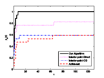
Figure 1 shows the performance profiles of the five solvers. The most
significant aspect of Figure 1 is that on this test set our algorithm
outperforms all other solvers. The performance profile for our algorithm lies
above all the others for all performance ratios. According to Figure 1, we
observe that our algorithm has shown to be substantially more efficient more
often than the three programs in KNITRO.
is the probability that
the solver will win over the rest of the solvers (Dolan and More', 2002).
Figure 1 shows the performance profiles of the five solvers. The most
significant aspect of Figure 1 is that on this test set our algorithm
outperforms all other solvers. The performance profile for our algorithm lies
above all the others for all performance ratios. According to Figure 1, we
observe that our algorithm has shown to be substantially more efficient more
often than the three programs in KNITRO.
4. Conclusion
We proposed a projected structured BFGS scheme for approximating the projected structured Hessian matrix in an exact penalty method for solving constrained nonlinear least squares problems. We established the local two-step superlinear convergence of the proposed algorithm. Comparative numerical results using the performance profile of Dolan and More' showed the efficiency and robustness of the algorithm.
Acknowledgements
The authors thank Iran National Science Foundation (INSF) for supporting this work under grant no. 88000800.
References
Bartels, R. H., Mahdavi-Amiri, N. (1986). On generating test problems for nonlinear programming algorithms. SIAM Journal of Scientific and Statistical Computing, 7(3), pp. 769–798. View Article
Bidabadi, N., Mahdavi-Amiri, N. (2012). A two-step superlinearly convergent projected structured BFGS method for constrained nonlinear least squares. To appear in Optimization View Article
Coleman, T. F., Conn, A. R. (1982a). Nonlinear programming via an exact penalty function: Asymptotic analysis. Mathematical Program., 24, pp. 123–136. View Article
Coleman, T. F., Conn, A. R. (1982b). Nonlinear programming via an exact penalty function: Global analysis. Mathematical Program., 24, pp. 137–161. View Article
Dennis, J. E., Martinez, H. J., Tapia R. A. (1989). Convergence theory for the structured BFGS secant method with an application to nonlinear least squares. Journal of Optimization Theory and Applications, 61, pp. 161-178. View Article
Dolan, E. D., More, J. J. (2002). Benchmarking optimization software with performance profiles. Math. Program., 91, pp. 201-213. View Article
Golub, G., Pereyra, V. (2003). Separable nonlinear least squares: the variable projection method and its applications, topical review. Inverse Problems 19, pp. R1–R26 View Article
Fletcher, R., Xu, C. (1987). Hybrid methods for nonlinear least squares. IMA Journal of Numerical Analysis, 7, pp. 371-389. View Article
Li, Z. F., Osborne, M. R., Prvan, T. (2002). Adaptive algorithm for constrained least-squares problems. Journal of Optimization Theory and Applications, 114(2), pp. 423-441. View Article
Mahdavi-Amiri, N., Ansari, M. R. (2012a). Superlinearly convergent exact penalty projected structured Hessian updating schemes for constrained nonlinear least squares: asymptotic analysis. To appear in Bulletin of the Iranian Mathematical Society, View Article
Mahdavi-Amiri, N., Ansari, M. R. (2012b). Superlinearly convergent exact penalty projected structured Hessian updating schemes for constrained nonlinear least squares: global analysis. To appear in Optimization View Article
Mahdavi-Amiri, N., Ansari, M. R. (2012c). A Superlinearly Convergent Penalty Method with Nonsmooth Line Search for Constrained Nonlinear Least Squares. SQU Journal for Science, 17(1), pp. 103-124. View Article
Mahdavi-Amiri, N., Bartels, R. H. (1989). Constrained nonlinear least squares: An exact penalty approach with projected structured quasi-Newton updates. ACM Transactions on Mathematical Software, 15(3), pp. 220–242 View Article
Mullen, K. M., Vengris, M., van Stokkum, I. H. M. (2007). Algorithms for separable nonlinear least squares with application to modeling time-resolved spectra. Journal of Global Optimization, 38, pp. 201–213 View Article
Nievergelt, Y. (2000). A tutorial history of least squares with applications to astronomy and geodesy. Journal of Computational and Applied Mathematics, 121, pp. 37-72. View Article
Nocedal, J., Overton, M. L. (1985). Projected Hessian updating algorithms for nonlinearly constrained optimization. SIAM Journal of Numerical Analysis, 22(5), pp. 821–850. View Article